Mastering sql query optimization techniques: Boost Your DB Performance
Discover sql query optimization techniques to speed up your queries, diagnose bottlenecks, and apply practical, real-world fixes that boost database performance.
When you get serious about SQL performance, you quickly realize it's a game of inches. It's about a systematic process of finding the slow spots, figuring out why they're slow, and then intelligently rewriting them to be faster and more efficient. The whole idea is to get your database to do less work, which means faster response times and a happier application.
Finding the Slow Queries That Are Sabotaging Your App
We've all been there. A single, poorly-written query can grind an entire application to a halt, leading to cascading failures and a terrible user experience. But finding that one bad actor in a sea of thousands of queries can feel overwhelming.
The trick isn't to guess or randomly tweak things. The professionals use a repeatable workflow to hunt down performance hogs. It’s all about using data to find the queries that consume the most resources—because those are the ones that will give you the biggest bang for your buck when you fix them.
It all starts with getting a baseline. You can’t know if you’ve made things better if you don’t know how bad they were to begin with. Before you change a single line of code, you need to measure how your query performs right now.
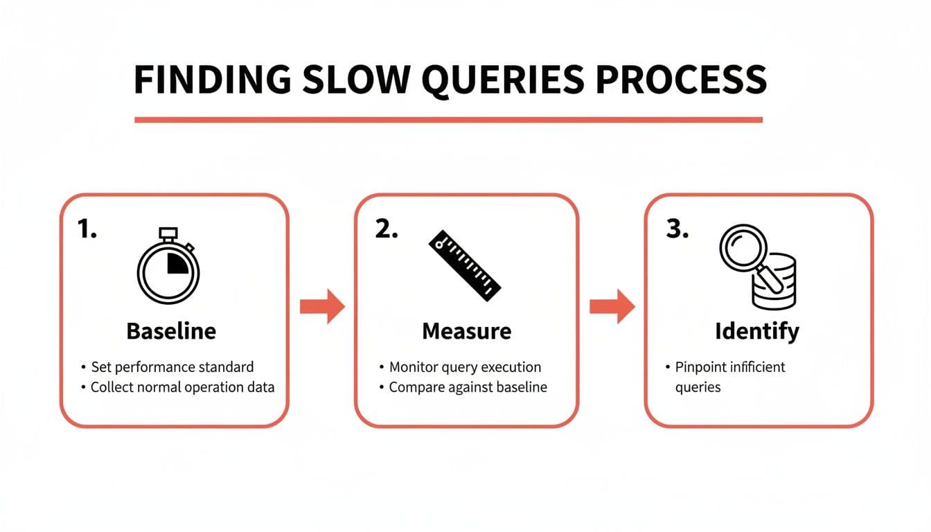
This workflow is your path from a vague sense that "the app is slow" to a concrete list of queries that need your immediate attention.
Establish a Performance Baseline
First things first: time the query. How long does it actually take to run? Most modern SQL clients and IDEs, including tools like TableOne, conveniently display the execution time right after you run something.
If you're in the command line, you have direct tools at your disposal:
- In PostgreSQL's
psqlclient, just type\timingbefore your query. It will automatically report the execution time. - In MySQL, you can enable profiling with
SET profiling = 1;to get detailed timing information.
The goal is simple: get a number. Is this query taking 50 milliseconds, 500 milliseconds, or a whopping 5 seconds? That single metric is the bedrock for everything that follows.
This initial diagnostic step is how you begin to separate the fast queries from the ones that are dragging you down.
Identify the True Bottlenecks
Okay, you have a baseline. Now for the real detective work: finding out why a query is slow. This is where the execution plan becomes your best friend. Think of it as a roadmap drawn by the database, detailing every step it plans to take to get your data. It’s the key to seeing whether it's using an efficient index or taking the slow road with a full table scan.
To get this roadmap, you simply put EXPLAIN in front of your query. Better yet, use EXPLAIN ANALYZE.
EXPLAINshows the estimated plan. It’s a quick, theoretical look at what the database thinks it will do, without actually running the query.EXPLAIN ANALYZEis where the magic happens. It runs the query and then gives you the plan alongside the actual time and row counts for each step. This is infinitely more useful for diagnosing real-world problems.
When you're looking at that output, you're hunting for red flags. The most common culprit? A Seq Scan (Sequential Scan) on a large table. This is the database's way of telling you it had to read every single row because it couldn't find a helpful index. Pinpointing these inefficient operations is the core of SQL query optimization—it tells you exactly where to focus your effort.
If you're just getting started and need help getting your environment set up, our guide on how to connect to a PostgreSQL database is a great place to begin.
For a quick reference, here's a checklist to run through when you first encounter a slow query.
Quick Diagnostic Checklist for Slow Queries
This table summarizes the initial diagnostic steps you can take across any major SQL database to start your investigation.
| Step | Action | Why It Matters | Tool/Command Example |
|---|---|---|---|
| 1. Baseline | Measure the query's raw execution time. | You need a starting number to know if your changes have any impact. | \timing (psql) or check your SQL client's output. |
| 2. Explain | Generate the query's execution plan. | This shows the database's intended strategy for fetching the data. | EXPLAIN SELECT ... |
| 3. Analyze | Run the query and get the actual plan and performance metrics. | This confirms the theoretical plan with real-world data, revealing true costs and row counts. | EXPLAIN ANALYZE SELECT ... |
| 4. Look for Scans | Identify Sequential Scan or Full Table Scan operations on large tables. | These are often the biggest performance killers and indicate a missing or unused index. | Check the EXPLAIN output for these keywords. |
By following this simple checklist, you move from guesswork to a structured, data-driven approach to fixing performance problems.
Learning to Read an Execution Plan Like a Pro
So, you’ve found a slow query. What's next? You need to figure out why it’s slow. For that, your single most powerful tool is the query execution plan. Think of it as the database's internal monologue, revealing the exact, step-by-step strategy it's using to fetch your data.
Learning to read this plan is the difference between guessing and knowing. By using commands like EXPLAIN and EXPLAIN ANALYZE, you can translate the database's strategy into real, actionable insights.
Decoding Common Plan Operations
At first glance, an execution plan can look like a wall of intimidating jargon. Don't worry. Once you learn to spot a few key terms, you'll find they tell a pretty clear story. These are the most common operations you'll run into.
-
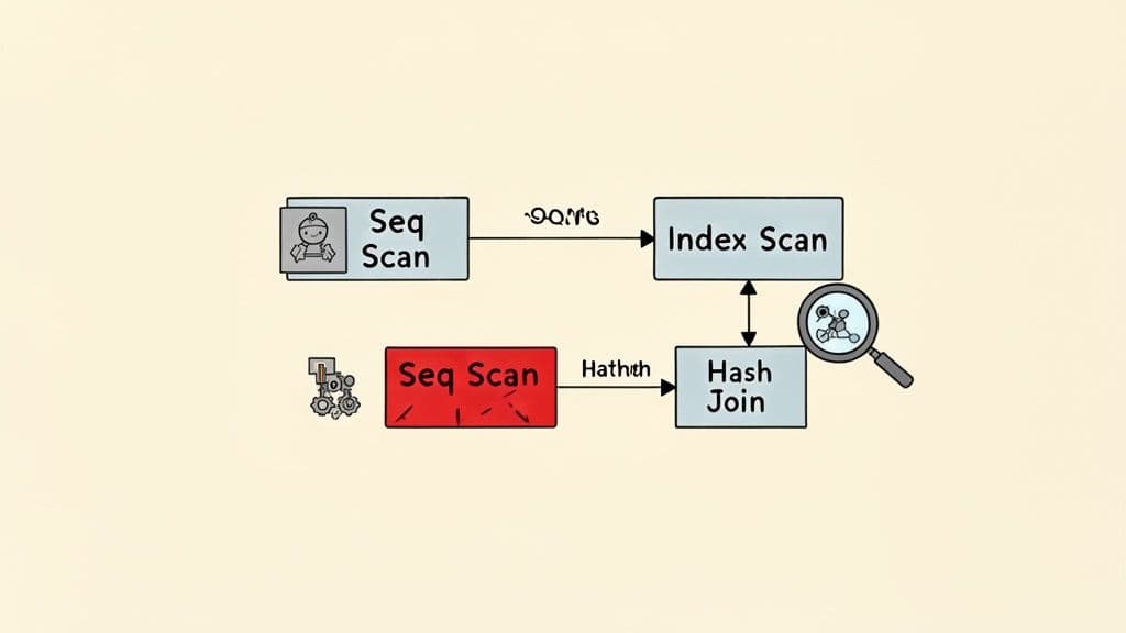
Sequential Scan (or Full Table Scan): This is the database reading every single row in a table from start to finish. For small tables, this is totally fine. But on a table with millions of rows, it's often a massive performance killer and a clear signal that you're missing an index.
-
Index Scan: The opposite of a sequential scan. This means the database is using an index to zero in on the exact rows it needs. For selective queries, this is what you want to see. It’s like using the index of a book instead of flipping through every page.
-
Nested Loop Join: The database loops through every row of the first table and, for each one, scans the second table to find matches. It’s efficient when one table is tiny, but it can be brutally slow if both tables are large.
-
Hash Join: The database builds an in-memory hash table from the smaller table, then reads the larger table and probes the hash table for matches. This is usually much faster than a nested loop when joining big tables.
Getting comfortable with these basic building blocks is the first real step toward diagnosing what’s wrong with a query.
An execution plan isn't just a report; it's a conversation with your database. When you see a
Seq Scanon a massiveuserstable to find one person by their email, the database is telling you, "I couldn't find a shortcut, so I did it the hard way."
That's your cue to give it that shortcut—almost always with an index.
Spotting Red Flags in an Execution Plan
A healthy plan is one where the database does the least amount of work possible. Two major red flags often point to trouble: full table scans on large tables and wildly inaccurate row estimates.
This is where the difference between EXPLAIN (the estimate) and EXPLAIN ANALYZE (the actual execution) becomes critical. If the planner estimates it will process 10 rows but actually processes 10 million, you have a huge problem. This kind of discrepancy often points to stale statistics, which forces the optimizer to make bad decisions, like choosing a nested loop when a hash join would have been lightyears faster.
A good SQL client can make digging through plans much easier. If you're looking for one, check out our guide on the best database client for tools that really simplify plan analysis.
Over the past decade, this entire process has become more dynamic. Modern databases have rolled out adaptive query optimization, which is a cornerstone of SQL performance management that allows for real-time adjustments. SQL Server’s adaptive join, for instance, can actually switch its join strategy mid-execution based on the real row counts it's seeing. This move from static planning to runtime intelligence is now common in systems from Oracle to Google BigQuery, and it explains why query performance can sometimes feel unpredictable. You can find more insights about these adaptive mechanisms in modern databases on arxiv.org.
Building an Intelligent Indexing Strategy
You've found a slow query, and the execution plan screams "full table scan." Your first thought is probably to slap a CREATE INDEX on it. That's a solid instinct, and often the right first move. But a truly effective indexing strategy is much more than just adding indexes—it's about choosing the right kind of index, designing it thoughtfully, and, just as importantly, knowing when to get rid of them.
This is where you'll find some of the biggest performance wins. An index is simply a special lookup table that the database can use to find rows quickly without having to comb through the entire dataset. It's like the index in the back of a book; you wouldn't read every single page to find a topic, would you? You'd just jump straight to the correct page.
Moving Beyond the Basic B-Tree
Out of the box, databases like PostgreSQL and MySQL default to a B-Tree index. It’s an absolute workhorse, fantastic for a wide range of comparisons like =, >, <, and BETWEEN. For most WHERE clauses filtering on standard data types like integers, text, or dates, a B-Tree is exactly what you need.
But modern databases have a whole toolbox of specialized indexes. Knowing when to pull out something other than a B-Tree is the mark of a seasoned pro.
- Hash Index: These are built for one job and one job only: pure equality checks (
=). They can be ridiculously fast for direct lookups but offer zero flexibility. Don't even think about using them for a range query. - GIN/GiST (PostgreSQL): These are where PostgreSQL really flexes its muscles. A GIN (Generalized Inverted Index) is a lifesaver for indexing composite values, like the elements in a
jsonbobject or an array. A GiST (Generalized Search Tree) is your go-to for more complex data types, like geometric data or for powering full-text search.
Picking the right index is like using the right tool. You could hammer in a nail with a screwdriver, but it’s going to be slow, messy, and frustrating.
The Critical Art of Multi-Column Indexes
It's rare for a query to filter on just a single column. More often, you're looking for something like active users who signed up within a certain date range. This is where multi-column indexes, also called composite indexes, are your best friend.
Let's say you have an e-commerce orders table and a query you run all the time:
SELECT * FROM orders
WHERE customer_id = 123
AND status = 'shipped';
You could create two separate indexes, one on customer_id and another on status. The database might use them, but it’s not very efficient. The far better solution is a single multi-column index: CREATE INDEX idx_orders_customer_status ON orders (customer_id, status);.
Now, here's the crucial part: the order of columns in a multi-column index matters immensely. An index on (customer_id, status) can be used perfectly for queries filtering on customer_id alone, or for queries filtering on both customer_id and status. But it's almost completely useless for a query that only filters on status.
A good rule of thumb is to put the column with the highest cardinality (the most unique values) first. In our example, there are far more unique
customer_idvalues thanstatusvalues, so(customer_id, status)is the clear winner.
This single, well-designed index can take a query from scanning millions of rows down to just a handful, cutting execution time from minutes to milliseconds. If you want to dive deeper into how this works, check out our guide on the composite key in SQL.
The Hidden Cost of Indexes
Indexes feel like magic for speeding up SELECT queries, but they aren't free. Every time you INSERT, UPDATE, or DELETE a row, the database has to do extra work. It updates the table data, and then it has to update every single index that points to it.
This means a table with a dozen indexes will have noticeably slower write performance. A common pitfall is to keep adding indexes reactively over the years without ever going back to see if they're still being used. Before you know it, your table is bloated with unused indexes that slow down every write operation for no reason.
Hunting down and dropping these unused indexes is a fantastic optimization trick. Most databases have built-in tools to help you with this:
- PostgreSQL: The
pg_stat_user_indexesview is your source of truth. It tracks usage statistics, including the number of index scans (idx_scan). A practical query to find unused indexes is:SELECT relname, indexrelname FROM pg_stat_user_indexes WHERE idx_scan = 0 AND schemaname = 'public';. If an index has zero scans after a good long while, it’s a strong candidate for deletion. - MySQL: Since version 8.0, you can query the
performance_schemato find index usage statistics and spot the ones that are just gathering dust.
Think of an index audit as cleaning out the garage. You clear out the clutter, free up valuable space, and make everything run a lot more smoothly. A smart indexing strategy is just as much about what you remove as what you add.
Rewriting Inefficient Queries for Peak Performance
A smart indexing strategy can solve a surprising number of performance issues. But what happens when you’ve added the perfect index and your query is still stubbornly slow? This usually means the query itself is written in a way that prevents the database from using its best tools.
Frankly, the most intuitive way to write a query often isn't the most efficient. This section is a playbook of common SQL anti-patterns and the rewrites that fix them. These transformations are some of the most powerful tools in your optimization toolkit because they guide the query planner toward a much faster execution path. You'll be surprised how small changes can lead to dramatic speed improvements.
Keep Your Indexed Columns Clean
Applying a function to a column in your WHERE clause is one of the most common performance traps I see. It makes the column "non-sargable," a technical term that just means the database can't use an index on it anymore.
Let's say you have a users table with a B-Tree index on the created_at timestamp. You want to find everyone who signed up today. It’s natural to write something like this:
The Anti-Pattern
SELECT user_id, email
FROM users
WHERE DATE(created_at) = '2023-10-27';
The problem here is the DATE() function. The database has no choice but to run that function on every single row before it can check the condition. This forces a full table scan, which is agonizingly slow on a large table.
The fix is to flip the logic around so the indexed column stands alone.
The Optimizer-Friendly Fix
SELECT user_id, email
FROM users
WHERE created_at >= '2023-10-27 00:00:00'
  AND created_at < '2023-10-28 00:00:00';
This new version allows the database to perform a highly efficient index range scan on the created_at column. This simple change can often cut query time from seconds down to milliseconds.
Replace OR with UNION ALL
The OR operator can be a real headache for query optimizers, especially when the conditions involve different columns. The planner might struggle to use multiple indexes effectively and could fall back to a much less efficient plan.
Imagine you're looking for products that are either low in stock or have been recently discontinued.
The OR Dilemma
SELECT product_id, product_name
FROM products
WHERE stock_count < 10 OR discontinued_date IS NOT NULL;
If you have separate indexes on stock_count and discontinued_date, the optimizer might only use one of them—or neither.
A better approach is to split this into two simpler queries and stitch the results together with UNION ALL.
The UNION ALL Strategy
SELECT product_id, product_name
FROM products
WHERE stock_count < 10
UNION ALL
SELECT product_id, product_name
FROM products
WHERE discontinued_date IS NOT NULL AND stock_count >= 10;
Now, each SELECT can use its own dedicated index. I've also added a condition to the second query to avoid pulling the same product twice. Using UNION ALL is also a key part of this trick—it's much faster than UNION because it doesn't waste time checking for and removing duplicate rows.
The principle is simple: break one complex problem that the optimizer struggles with into two simpler problems that it can solve very efficiently.
This rewrite often results in a plan that uses two fast index scans instead of one slow table scan.
Unwind Correlated Subqueries into JOINs
A correlated subquery is a subquery that depends on the outer query for its values. It’s the SQL equivalent of nesting a for loop inside another for loop, and it's a notorious performance killer. For every single row processed by the outer query, the inner subquery has to be executed all over again.
Let's say you want to find all orders placed by customers from California.
The Correlated Subquery Nightmare
SELECT o.order_id, o.order_date
FROM orders o
WHERE 'California' = (
  SELECT c.state
  FROM customers c
  WHERE c.customer_id = o.customer_id
);
If your orders table has 1 million rows, that inner query is going to run 1 million times. Ouch.
The solution is almost always to rewrite the query using a JOIN. Modern optimizers are getting better at fixing this automatically, but writing it explicitly is safer and, in my opinion, much more readable.
The Performant JOIN
SELECT o.order_id, o.order_date
FROM orders o
JOIN customers c ON o.customer_id = c.customer_id
WHERE c.state = 'California';
This version allows the database to use indexes on both o.customer_id and c.customer_id, pick the best join strategy (like a hash join), and filter the results efficiently in one go. The performance difference can be astronomical, and mastering this kind of rewrite is essential for anyone working with large datasets.
Going Beyond the Query: Advanced Optimization Strategies
So you've perfected your indexes and rewritten your queries, but your application is still sluggish. What now? This is the point where we have to zoom out from the individual query and look at the bigger picture. We're moving beyond micro-level fixes and into macro-level architectural strategies.
When simple rewrites aren't enough, it’s a sign that the problem might be rooted deeper—in your database schema, server configuration, or overall data access patterns. This is where you transition from being a query tuner to thinking like a database architect, making changes that deliver lasting performance gains.
Revisit Your Schema Design
The way you structure your tables—your schema—has a massive impact on performance. The textbook approach is normalization, where you split data into related tables to eliminate redundancy. Think separating customer info from their orders. This is great for keeping data consistent and makes write operations clean and efficient.
But what happens in read-heavy applications, like an analytics dashboard? All those JOIN operations needed to piece a normalized schema back together can become a serious bottleneck. This is where a little bit of denormalization can be a lifesaver. It’s the deliberate choice to add redundant data back into your tables specifically to speed up reads.
Let’s take a social media app as an example. You need to show a username next to every post.
- Normalized approach: Every time you fetch posts, you
JOINthepoststable with theuserstable onuser_id. - Denormalized approach: You store the
usernamedirectly in thepoststable right alongside theuser_id.
That simple change eliminates the JOIN entirely, making your post feed load much faster. The catch? If a user updates their username, you now have to update it in the users table and in every single one of their posts.
Denormalization is a strategic trade-off. You’re accepting slower, more complex writes in exchange for lightning-fast reads. It's a powerful tool, but use it wisely—it’s best for data that’s read constantly but rarely changes.
Pre-Calculate Results with Materialized Views
Some queries are just naturally slow and complex. Imagine generating a monthly sales report that has to aggregate millions of transactions with multiple joins and calculations. Running that on-demand is a recipe for a database meltdown.
This is a perfect job for a materialized view. Unlike a standard view (which is just a stored query), a materialized view actually runs the query and stores the result as a physical table. When you query the materialized view, you’re just reading from this pre-built cache. It's incredibly fast.
In PostgreSQL, creating one is simple:
CREATE MATERIALIZED VIEW monthly_sales_summary AS
SELECT
    date_trunc('month', order_date) AS sales_month,
    product_category,
    SUM(sale_amount) AS total_sales
FROM sales
GROUP BY 1, 2;
Querying monthly_sales_summary is now almost instant. The trade-off, of course, is that the data can become stale. You have to periodically run REFRESH MATERIALIZED VIEW to update it, which is typically done on a nightly schedule or another low-traffic window.
Partition Large Tables
When a single table swells to hundreds of millions or even billions of rows, performance can degrade even with good indexes. A table just becomes too massive to manage efficiently. Table partitioning is a fantastic technique for dealing with this by breaking one huge logical table into smaller, more manageable physical chunks.
A classic use case is partitioning a massive events table by month. When you run a query for events in a specific month, the database is smart enough to scan only the partition for that month, completely ignoring all the others. For time-series data, this is a game-changer.
Tweak Your Database Configuration
Sometimes the problem isn't your query or your schema—it's the server itself. Every database has a ton of configuration knobs that control how it uses resources like memory and disk I/O. The default settings are designed to be safe and run anywhere, but they are rarely optimal for your specific workload.
Here are two key settings you should absolutely know:
work_mem(PostgreSQL): Controls how much memory can be used for sorting and hashing before the database gives up and starts writing temporary files to disk. For complex analytical queries, bumping this up can prevent slow disk I/O and dramatically improve performance.innodb_buffer_pool_size(MySQL): This is the holy grail of MySQL performance. It defines the memory cache for your InnoDB table and index data. On a dedicated database server, it's common practice to set this to 50-75% of the total system RAM to keep as much of your hot data in memory as possible.
The Rise of AI in Query Optimization
The future of these advanced techniques points toward less manual tinkering and more intelligent automation. AI and machine learning are already starting to shift SQL optimization from a human-driven, rule-based process to a more data-driven one. These systems can analyze performance data from thousands of queries to spot patterns and find better execution plans than a traditional optimizer ever could.
This trend is visible in products like Microsoft SQL Server 2025 and its Intelligent Query Processing. For those of us using modern database clients like TableOne to connect to PostgreSQL and MySQL, it means performance will increasingly rely on the database engine's own ability to learn and adapt. You can read more about how AI is reshaping SQL performance to get a glimpse of what's coming next.
Common Questions on SQL Performance Tuning
As you start applying these optimization techniques, you'll naturally run into some common questions and tricky situations. This section tackles the practical, real-world problems developers bump into every day when trying to squeeze every last drop of performance from their databases. Consider it your quick-reference guide for those "what-if" moments.
How Do I Know if My Index Is Actually Being Used?
You can't just assume an index is working; you have to ask the database. The only way to be certain is to run your query with EXPLAIN ANALYZE and look closely at the execution plan.
What you’re hoping to see are operations like an Index Scan or an Index-Only Scan. If you spot a Seq Scan (Sequential Scan) on a large table where you expected an index to kick in, that's a major red flag. It means the optimizer decided reading the entire table was a better idea than using your index.
This usually happens for a few classic reasons:
- You’re using a function on the indexed column (like
WHERE lower(email) = '...'), which makes it non-sargable. - The index statistics are out of date, causing the planner to make a poor choice.
- Your query isn't very selective and pulls back such a large percentage of the table that a full scan is, in fact, faster.
Can Adding Too Many Indexes Hurt Performance?
Absolutely. Indexes are a perfect example of a trade-off in database design. They work wonders for speeding up SELECT queries, but they add overhead to every single write operation—INSERT, UPDATE, and DELETE.
Each time data is written, the database has to update not just the table but also every relevant index. If you have a write-heavy table with a bunch of unnecessary indexes, you can create a serious performance bottleneck. It's a constant balancing act between read speed and write speed.
A mature optimization strategy isn't just about adding indexes. It's also about periodically auditing for and removing the ones that are no longer used. This simple housekeeping can reclaim performance you didn't even realize you were losing.
What Is the Difference Between EXPLAIN and EXPLAIN ANALYZE?
This is a crucial distinction. EXPLAIN gives you the estimated execution plan. It's the database's best guess, based on internal statistics, of how it will run the query. The key thing is, it doesn't actually run anything. It's fast and provides a theoretical roadmap.
EXPLAIN ANALYZE, on the other hand, is much more powerful. It first executes the query and then shows you the plan, complete with the actual execution times and row counts for each step. This is invaluable for troubleshooting because it reveals exactly where the planner's estimates went wrong.
If you see a massive gap between the estimated row count and the actual row count, that’s a huge clue. It almost always means your database statistics are stale, leading the optimizer down the wrong path.
When Should I Use a Subquery Versus a JOIN?
These days, modern SQL optimizers are pretty smart and can often rewrite many subqueries into more efficient JOINs behind the scenes. That said, as a general rule, an explicit JOIN is usually more readable and gives the planner clearer instructions to work with.
The one you really need to watch out for is the correlated subquery. This is a performance killer where the inner query runs once for every single row of the outer query. These should almost always be rewritten as a JOIN.
When in doubt, there's a simple, foolproof method: test both versions with EXPLAIN ANALYZE. Let the real-world performance data tell you which approach is truly better for your specific database and data set.
Managing queries and optimizing performance across different databases like PostgreSQL, MySQL, and SQLite can be a real challenge. With TableOne, you get a single, modern tool to browse tables, edit data, run queries, and even compare database schemas—all with a simple, one-time license.